• Nov. 14, 2021, 1:25 a.m.

    Background

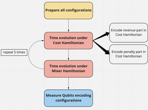
    In this post, we will discuss how to implement a quantum circuit that solves an optimization problem without classical optimization, based on this adiabatic quantum computation framework. In other words, the circuit gives a good approximate solution in a single run. This is contrary to the well-known QAOA quantum-classical hybrid approach.

    (The following answers are also solutions to 2021 Qiskit Fall Challenge Problem 4c)

    Battery Revenue Optimization Problem

    Battery storage systems have provided a solution to flexibly integrate large-scale renewable energy (such as wind and solar) in a power system. The revenues from batteries come from different types of services sold to the grid. The process of energy trading of battery storage assets is as follows: A regulator asks each battery supplier to choose a market in advance for each time window. Then, the battery operator will charge the battery with renewable energy and release the energy to the grid depending on pre-agreed contracts. The supplier therefore makes forecasts on the return and the number of charge/discharge cycles for each time window to optimize its overall return.

    How to maximize the revenue of battery-based energy storage is a concern of all battery storage investors. Choosing to let the battery always supply power to the market which pays the most for every time window might be a simple guess, but in reality, we have to consider many other factors.

    What we can not ignore is the aging of batteries, also known as degradation. As the battery charge/discharge cycle progresses, the battery capacity will gradually degrade (the amount of energy a battery can store, or the amount of power it can deliver will permanently reduce). After a number of cycles, the battery will reach the end of its usefulness. Since the performance of a battery decreases while it is used, choosing the best cash return for every time window one after the other, without considering the degradation, does not lead to an optimal return over the lifetime of the battery, i.e. before the number of charge/discharge cycles reached.

    Therefore, in order to optimize the revenue of the battery, what we have to do is to select the market for the battery in each time window taking both the returns on these markets (value), based on price forecast, as well as expected battery degradation over time (cost) into account.

    Problem Setting

    Here, we have referred to the problem setting in de la Grand'rive and Hullo's paper [1].

    Considering two markets $M_{1}$ , $M_{2}$, during every time window (typically a day), the battery operates on one or the other market, for a maximum of $n$ time windows. Every day is considered independent and the intraday optimization is a standalone problem: every morning the battery starts with the same level of power so that we don’t consider charging problems. Forecasts on both markets being available for the $n$ time windows, we assume known for each time window $t$ (day) and for each market:

    • the daily returns $\lambda_{1}^{t}$ , $\lambda_{2}^{t}$

    • the daily degradation, or health cost (number of cycles), for the battery $c_{1}^{t}$, $c_{2}^{t}$

    We want to find the optimal schedule, i.e. optimize the lifetime return with a cost less than $C_{max}$ cycles. We introduce
    image.png

    We introduce the decision variable $z_{t}, \forall t \in [1, n]$ such that $z_{t} = 0$ if the supplier chooses $M_{1}$ , $z_{t} = 1$ if choose $M_{2}$, with every possible vector $z = [z_{1}, ..., z_{n}]$ being a possible schedule. The previously formulated problem can then be expressed as:

    image.png

    Author Introduction

    Yusheng Zhao, graduated from Physics and Astronomy Master Program of Stony Brook University in 2020. He enjoys coding and learning about quantum computing. He achieved Top 10 scores in IBM Quantum Challenge Fall 2021 among over 1,200 participants.

    image.png

    PNG, 11.3 KB, uploaded by Editor on Nov. 14, 2021.

    image.png

    PNG, 3.0 KB, uploaded by Editor on Nov. 14, 2021.

  • bookmark

    Thread has been pinned globally.

  • Members 1 post
    Nov. 15, 2021, 10:32 a.m.

    Introduction

    In this post, I will describe how to solve Problem 4 C in IBM's Quantum Challenge Fall 2021. I need to thank my advisor, Prof. Tzu-Chieh Wei, from Stony Brook University for helping me test and improve my code.

    Contents

    Implementation Steps

    As described in the introduction post, optimization of the parameters for each layer of evolution is taken care of by IBM. We will be using a fixed set of parameters. We will only need to implement the time evolution of $H_{C}$ and $H_{M}$ with QuantumCircuit.

    image (3).png

    Cost Hamiltonian

    The general idea is to construct a Hamiltonian whose eigenenergy $\propto\sum_{t}\lambda^{t}_{i} + cost(z)$. In ref [1], this is achieved by dividing the Hamiltonian into return and penalty part.

    1. Return

      In this step, we encode the revenue information into the energy of eigenstates of $H_{C}$.

      When the $i_{th}$ qubit is measured to be in $\ket{0}$, we denote it as choosing to supply $M_{1}$ on day $i$. Similarly, the measured value of $\ket{1}$ will be choosing to supply electricity to $M_{2}$. To encode the revenue $\lambda_{i}$ into $H_{C}$, it suffices to make return part of $H_{C} \propto \otimes_{i} \sigma_{Z}^{i}$. Time evolution of the return part of $H_{C}$ would be equivalent to applying different phases on each qubit conditioned on the state it is in. E.g, if it's in $\ket{1}$, you apply a phase of $e^{-i \gamma p_{1}}$. If it's in $\ket{0}$, you apply a phase of $e^{-i \gamma p_{0}}$. However, this could not be achieved using a simple unitary gate on each qubit. As an alternative way, we could shift the revenue of $M_{1}$ to zero. Consequently, a phase gate of angle $\propto \lambda_{2} - \lambda_{1}$ is needed on each qubit. This way, only when the qubit is in $\ket{1}$, we apply a phase. The relative phase difference is preserved. This will be a hint to how we could simplify adding the degradation for each choice later.

    2. Penalty

      In this step, we encode the cost information into the energy eigenstates of $H_{C}$.

      To encode this cost information into the $H_{C}$, it is necessary to compute the sum of all costs over $t$ days for a specific configuration. We then “compare” the total cost to $C_{max}$. We could divide them into two tasks. Firstly, compute the cost. Secondly, flag the appropriate configurations and "add" penalty terms.

      2.1. Cost Calculation

      In this part, we will need to add up all cost values for $t$ days for all possible choices of supplying markets. If the steps are too long, you may just read the line after "Goal" to get the gist of each step.

      This is achieved in the following steps:

      1) Goal: Prepare all possible configurations.

      In a quantum register, index register, prepare $t$ qubits in all $2^{t}$ computational basis states. Each state will correspond to a possible choice of the market during the $t$ days.

      2) Goal: For each computational basis state, compute the corresponding cost value by adding up the cost value for each day in the chosen market.

      3) Goal: implement Draper QFT Adder

      To perform the addition, IBM proposed the use of Draper QFT Adder[2]. Another quantum register, denoted as data register, is used to store the sum of all costs during $t$ days. In order to compute the added cost value, a Quantum Fourier Transform is required to encode a number from its binary form encoded in qubits in data register into the relative phases of qubits in the same register. Following the QFT, phase gates of appropriate values are applied on each qubit to perform the addition of two numbers in the relative phases. After the addition, an inverse Quantum Fourier Transform is performed to retrieve the summed value from relative phases in the data register and encode them back into the computational basis in the data register.

      4) Goal: Apply addition based on configuration represented by qubits in index register

      Notice we will need to add different cost values based on the configuration in index register. A controlled version of step (3) is then applied on the data register. It is applied on the condition that the index register qubits’ values correspond to the configuration that requires the addition of that cost value on the total cost. E.g, when the $i_{th}$ qubit value is $\ket{1}$, you perform step (3) with added value of $c_{i}$ from $M_{2}$. Since the values of qubits in the index register are in a superposition of all possible computational basis states, we will need a controlled unitary to achieve this. In terms of Qiskit language, we could make the step (3) a gate. Then construct the controlled version of that gate using .control(). This step is illustrated by Fig. 9 in [1].

      5) Goal: Flag configurations that exceed $C_{max}$.

      After the summation of cost values, we need to flag the configurations that exceed the $C_{max}$ total cost limit. This could be achieved by shifting the total values of all configuration degradation costs and $C_{max}$ by a value of diff,($diff = 2^w - C_{max}$). After the shift, we have $C_{max} = 2^{w}$. In qubit representation, the $w_{th}$ qubit in data register will be 1 for $C_{max}$. Any total cost value with $w_{th}$ or higher qubit in state $\ket{1}$ exceeds the $C_{max}$ limit. We will need to turn another qubit in the flag register to $\ket{1}$ for this case. A multi-CNOT gate is used to achieve this effect with control qubits being $w_{th}$ and higher qubits in the data register.

      6) Goal: Apply penalty in terms of energy in $H_{C}$ for configurations flagged in last step.

      For all configurations that exceed $C_{max}$, we add $cost(z) - C_{max}$ to their eigenvalues in $H_{C}$. This is achieved by applying a controlled phased gate on each of the $i_{th}$ qubit in data register with an angle $2^{i}$.
      Following that, we will need to apply a phase gate with angle $C_{max}$ on the flag qubit. This is illustrated by Fig. 13 in [1].

      7) Goal: reinitialize data register and flag register for later use.

      Finally, we will reinitialize the data register and flag register into a clean state. This could be achieved by applying the steps of (3) and (5) in reverse.

    Mixer Hamiltonian

    In this step, we construct a circuit to apply the time evolution of a mixer Hamiltonian on the index register qubits.

    In general, the mixer Hamiltonian will need to be non-commuting to $H_{C}$. We use the good-old mixer Hamiltonian $H_{M}= \sum_{i}\sigma_{i}^{x}$. To implement the evolution of qubits under this Hamiltonian, we perform a rotation around the Pauli-X axis on each qubit.

    Improvement 1:

    Notice in step (3), QFT and inverse QFT is applied in each summation. However, this is a complete waste of a performance. Since we will do $t$ times of addition, the inverse QFT of $i_{th}$ addition could be canceled with QFT of $(i+1)_{th}$ addition. Doing so would save the cost of many QFT and IQFT.

    Improvement 2:

    Notice when we computed the total revenue, we only encoded the difference in revenue on the day $i$ for the two markets. This simplification could be repeated when summing up the cost values of all configurations. We could make the lowest configuration have a cost of $0$. Since we are guaranteed that the cost of two markets will be such that $c_{1}^{i} < c_{2}^{i}$, we could make the degradation of $M_{1}$ all zero. This would effectively make the lowest configuration have a total cost of 0. In step (3), we will no longer need to add $c_{1}^{i}$ since they are all zero. Doing so would also require a much smaller data register, since the sum of all costs is lowered by $\sum_{i}c_{1}^{i}$. Therefore, we will be saving a lot in QFT, IQFT, and other related calculations.

    Minor Improvements:

    • We could NOT encode the first cost values from $M_{1}$ and $M_{2}$ directly in the data register qubits. Previously I did so without realizing that this step does not commute with the later Mixer Hamiltonian's time evolution! THIS IS WRONG! DO NOT FOLLOW! Instead, we have to add all costs in the '''cost_calculation()'''. I will update the github link at the end to reflect this change. Please let me know if you would also like to have the functions provided by IBM and then modifed by me to test if each step is done correctly.
    • In step (3), we make $C_{max} = 2^{w}$. If the maximum degradation value is no larger than $2^{w} -1$, we could further reduce the size of the data register to $w+1$ qubits. And the flagging step (5) will not need a multi-CNOT. A single CNOT will suffice.
    • I found it helpful to transpile quantum circuits returned in each function. With parameter, optimization_levl=2 it will reduce your circuit cost.

    Further Discussion:

    • I am not sure how the best score manages to have a score of 50k. Using the process described above, you should comfortably reach a score of around 270k.
      Perhaps they did not use QFT Adder.
    • My Score:
      score.png
    • You may find the source code in this link. Please pardon my poor naming schemeand general lack of code aesthetics. I was focusing on speed of implementation.
    • I have also added testers in the same folder as the python script. Please see the notebook I upload for how to use them. They should help you verify whether your QFT adder, qubit reinitialization, and flagging process are implemented correctly

    References

    [1]: [de la Grand’rive and Hullo, 2019] de la Grand’rive, P. D. and Hullo, J.-F. (2019). Knapsack Problem variants of QAOA for battery revenue optimisation. arXiv:1908.02210 [quant-ph].

    [2]: [Draper, 2000] Draper, T. G. (2000). Addition on a Quantum Computer. arXiv:quant-ph/0008033.

    image (3).png

    PNG, 132.9 KB, uploaded by querystorm on Nov. 15, 2021.

    flowchart.png

    PNG, 148.6 KB, uploaded by exAClior on Nov. 15, 2021.

    score.png

    PNG, 108.0 KB, uploaded by exAClior on Nov. 15, 2021.